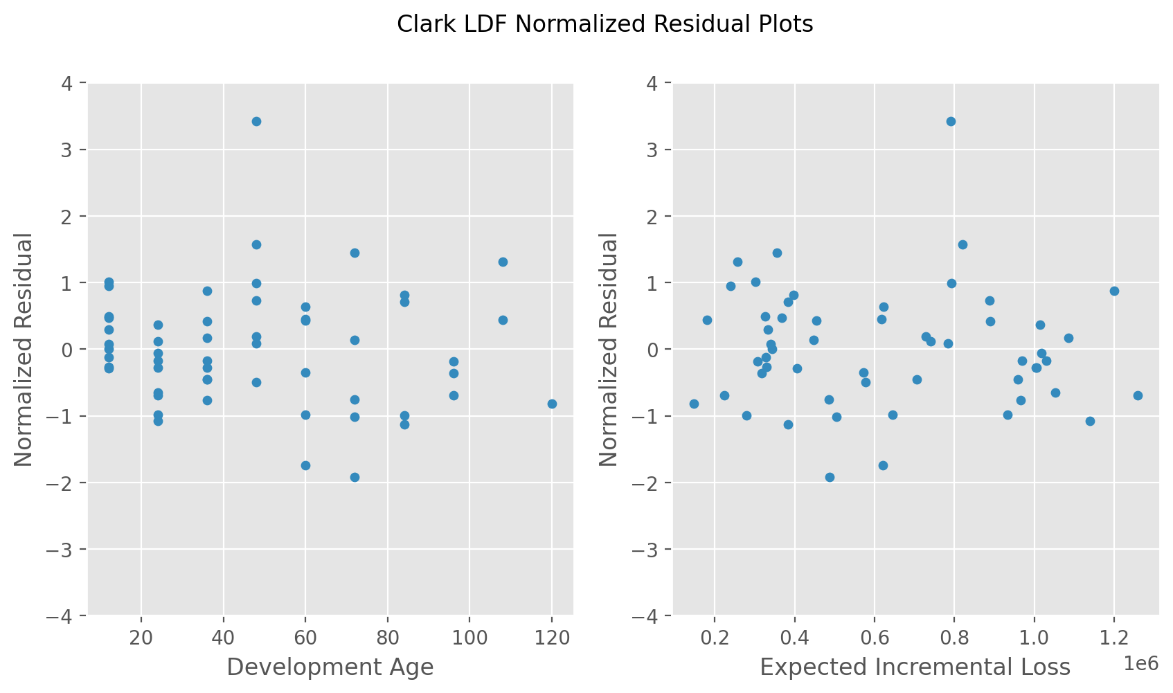
Clark Residual Plots

import chainladder as cl

This example demonstrates how to recreate the normalized residual plots in Clarks LDF Curve-Fitting paper (2003).

# Fit the basic model
genins = cl.load_sample("genins")
genins = cl.ClarkLDF().fit(genins)

# Grab Normalized Residuals as a DataFrame
norm_resid = genins.norm_resid_.melt(
    var_name="Development Age", value_name="Normalized Residual"
).dropna()

# Grab Fitted Incremental values as a DataFrame
incremental_fits = genins.incremental_fits_.melt(
    var_name="Development Age", value_name="Expected Incremental Loss"
).dropna()
incremental_fits = incremental_fits.merge(
    norm_resid, how="inner", left_index=True, right_index=True
)

Show code cell source

Hide code cell source

import matplotlib.pyplot as plt

plt.style.use("ggplot")
%config InlineBackend.figure_format = 'retina'

# Plot the residuals vs Age and vs Expected Incrementals
fig, ((ax0, ax1)) = plt.subplots(ncols=2, figsize=(10, 5))

# Left plot
norm_resid.plot(
    x="Development Age",
    y="Normalized Residual",
    kind="scatter",
    grid=True,
    ylim=(-4, 4),
    ax=ax0,
)
# Right plot
incremental_fits.plot(
    x="Expected Incremental Loss",
    y="Normalized Residual",
    kind="scatter",
    grid=True,
    ylim=(-4, 4),
    ax=ax1,
)
fig.suptitle("Clark LDF Normalized Residual Plots");