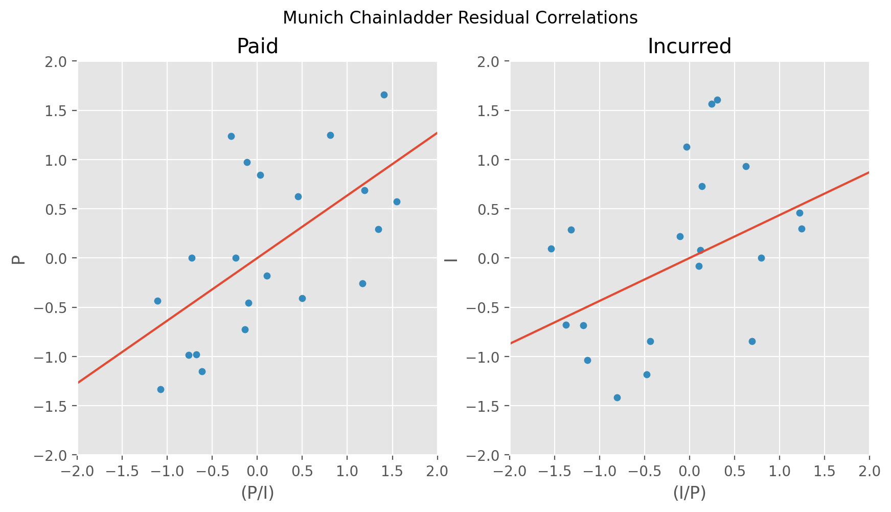
MunichAdjustment Correlation

import chainladder as cl
import pandas as pd
import numpy as np

This example demonstrates how to recreate the the residual correlation plots of the Munich Chainladder paper.

# Fit Munich Model
mcl = cl.load_sample("mcl")
model = cl.MunichAdjustment([("paid", "incurred")]).fit(mcl)

# Paid lambda line
paid_lambda = pd.DataFrame({
    "(P/I)": np.linspace(-2, 2, 2),
    "P": np.linspace(-2, 2, 2) * model.lambda_.loc["paid"],
})

# Paid scatter
paid_plot = pd.concat(
    (
        model.resids_["paid"].melt(value_name="P")["P"],
        model.q_resids_["paid"].melt(value_name="(P/I)")["(P/I)"],
    ),
    axis=1,
)

# Incurred lambda line
inc_lambda = pd.DataFrame({
    "(I/P)": np.linspace(-2, 2, 2),
    "I": np.linspace(-2, 2, 2) * model.lambda_.loc["incurred"],
})

# Incurred scatter
incurred_plot = pd.concat(
    (
        model.resids_["incurred"].melt(value_name="I")["I"],
        model.q_resids_["incurred"].melt(value_name="(I/P)")["(I/P)"],
    ),
    axis=1,
)

Show code cell source

Hide code cell source

import matplotlib.pyplot as plt

plt.style.use("ggplot")
%config InlineBackend.figure_format = 'retina'

# Plot Data
fig, ((ax0, ax1)) = plt.subplots(ncols=2, figsize=(10, 5))

paid_lambda.plot(x="(P/I)", y="P", legend=False, ax=ax0)
paid_plot.plot(
    kind="scatter", y="P", x="(P/I)", ax=ax0, xlim=(-2, 2), ylim=(-2, 2), title="Paid"
)

inc_lambda.plot(x="(I/P)", y="I", ax=ax1, legend=False)
incurred_plot.plot(
    kind="scatter",
    y="I",
    x="(I/P)",
    ax=ax1,
    xlim=(-2, 2),
    ylim=(-2, 2),
    title="Incurred",
)
fig.suptitle("Munich Chainladder Residual Correlations");