MunichAdjustment Basics

import chainladder as cl
import pandas as pd

This example demonstrates how to adjust LDFs by the relationship between Paid and Incurred using the MunichAdjustment.

# Load data
mcl = cl.load_sample("mcl")

# Traditional Chainladder
cl_traditional = cl.Chainladder().fit(mcl).ultimate_

# Munich Adjustment
dev_munich = cl.MunichAdjustment(paid_to_incurred=("paid", "incurred")).fit_transform(
    mcl
)
cl_munich = cl.Chainladder().fit(dev_munich).ultimate_

plot1_data = cl_munich.to_frame().T.rename(
    {"incurred": "Ultimate Incurred", "paid": "Ultimate Paid"}, axis=1
)

plot2_data = pd.concat(
    (
        (cl_munich["paid"] / cl_munich["incurred"])
        .to_frame(origin_as_datetime=False)
        .rename(columns={"2261": "Munich"}),
        (cl_traditional["paid"] / cl_traditional["incurred"])
        .to_frame(origin_as_datetime=False)
        .rename(columns={"2261": "Traditional"}),
    ),
    axis=1,
)

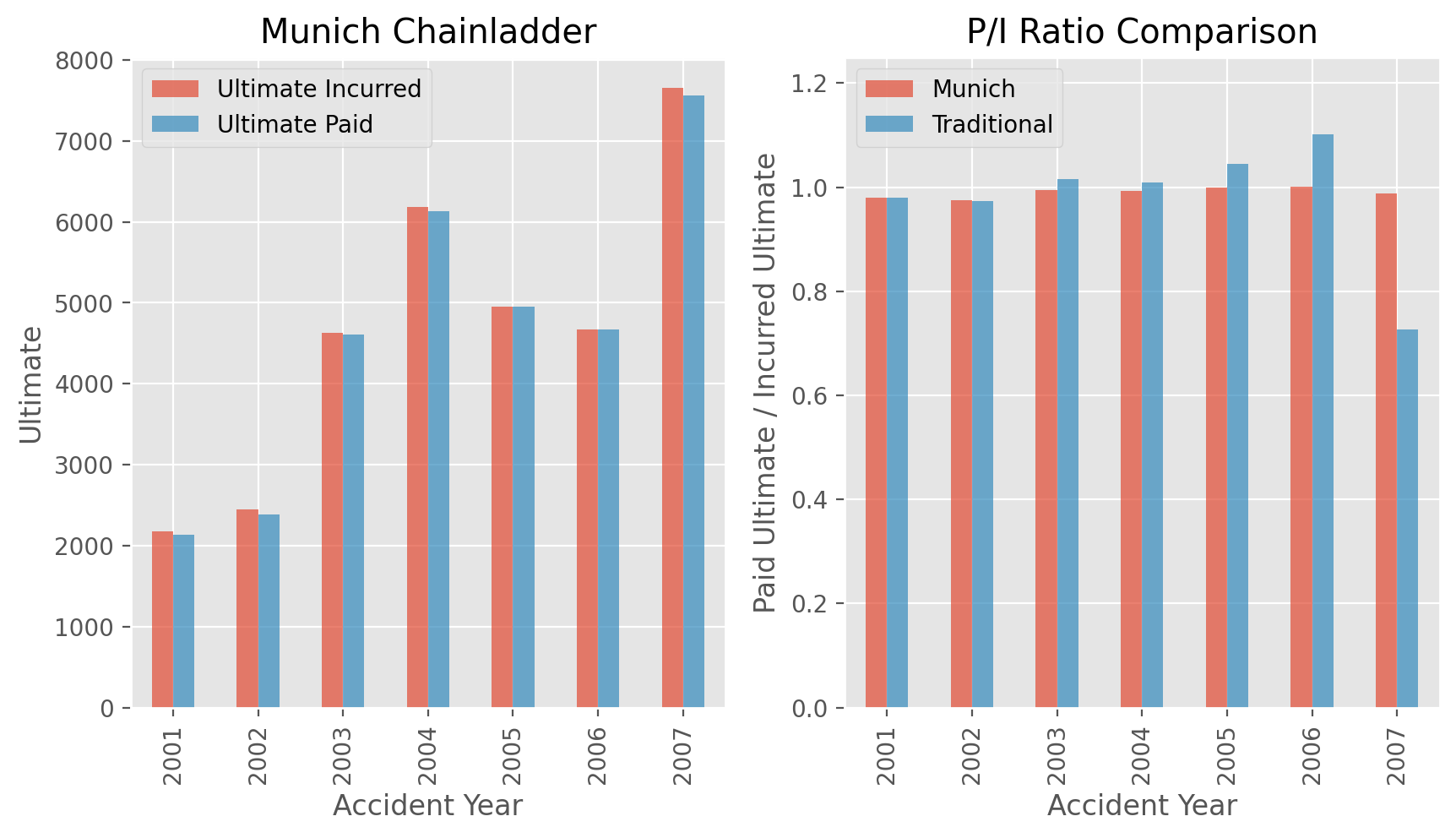
We can see how the Paid / Incurred Ultimates stay close to 1.0 for all origin periods under the MunichAdjustment while they diverge under the traditional Development.

Show code cell source

Hide code cell source

import matplotlib.pyplot as plt

plt.style.use("ggplot")
%config InlineBackend.figure_format = 'retina'

# Plot data
fig, (ax0, ax1) = plt.subplots(ncols=2, sharex=True, figsize=(10, 5))
plot_kw = dict(kind="bar", alpha=0.7)

plot1_data.plot(title="Munich Chainladder", ax=ax0, **plot_kw).set(
    ylabel="Ultimate", xlabel="Accident Year"
)
plot2_data.plot(title="P/I Ratio Comparison", ax=ax1, ylim=(0, 1.25), **plot_kw).set(
    ylabel="Paid Ultimate / Incurred Ultimate", xlabel="Accident Year"
);